Learning about GNU Radio - How the impedance tester works
A program doing mostly what computers do best - math.
Learning about GNU Radio - Table of Contents
Some time back, I described how I manually measure impedance on those rare occasions when I need to measure an inductor or capacitor.
It’s nothing really more than an application of the math involved in a voltage divider.
The example circuit in the last post is nothing more than a voltage divider connected to some audio cables.
Here’s the drawing again:
| Just a voltage divider |
|---|
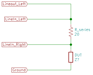 |
Written for the circuit above, the voltage divider formula looks like this:
$V_{LineIn \text{_} Right} = \frac{Z_{DUT} * V_{LineIn \text{_} Left}}{Z_{R \text{_} series} + Z_{DUT}}$
Rearranged to find the impedance of the device under test (DUT) it looks like this:
$Z_{DUT} = \frac{Z_{R \text{_} series}}{\frac{V_{LineIn \text{_} Left}}{V_{LineIn \text{_} Right}} - 1}$
To measure impedance at one frequency, you apply a signal with the desired frequency to $LineOut \text{_} Left$, measure at $LineIn \text{_} Left$ and $LineIn \text{_} Right$, do a little math and you’re done.
Well, not quite. The goal here is to measure the impedance of a speaker across the entire audio spectrum - from down near DC to over 20 kHz.
You can do the manual measurements a few times and plot the results to get an idea of the impedance across the whole range, but if you want a really detailed plot you’ll have to do that hundreds (if not thousands) of times. It’d take forever, and it’d be no fun at all.
Fortunately, computers are good at math and good at doing things repeatedly. This needs both. Repeatedly doing math.
The obvious way to do this is to have the computer generate sine waves at various frequencies, then measure the voltages, do the math, plot points, repeat until done.
I did in fact do that many years ago with a computer controlled signal generator and a computer controlled voltmeter. It was slow, but it worked. It did what I needed until I could get hold of something better. I don’t have that program any more, and couldn’t use it if I did have it. It misused a Motorola R2600 communications system analyser as an audio signal generator and AC voltmeter.
The better way to attack the problem is to generate a sweep that runs the whole range of frequencies in a fraction of a second. You capture the voltages over the entire period and apply a Fourier transformation to get the voltage for each frequency for a block of measurements in one go.
The down side there is that you have to have the measurement synchronized with the generator. Once a long time ago, I had access to a Stac AD416 data acquisition card that could do that very trick. You sent a chirp (frequency sweep) out through the built in digital to analog converter (DAC) in a block, and it could hand you back a block of data from the analog to digital converters (ADC) that exactly contained the time period of your chirp. I “built” a very nice impedance tester with the AD416 and LabView. It worked quite well, and I used it to solve a nasty problem with impedances that we had at work.
Without that synchronization, you get your chirp spread over multiple blocks of data for your Fourier spectrum analysis. That chops things up, and you get some seriously messed up measurements. Been there, done that, it isn’t useful.
PC sound cards don’t have that ability, and implementing a work around for it is ugly. Way more work than I’m going to do in the evenings after spending all day programming.
The alternative to a chirp is white noise. White noise (strictly speaking, band width limited white noise) contains all frequencies simultaneously. Over time, all frequencies are equally represented at the same average intensity.
This is the solution that I chose for this impedance tester.
The impedance tester generates white noise, and does two Fourier transforms - one for the applied signal and one for the signal as attenuated by the speaker. With the Fourier results in hand, you do the math to calculate the impedance for each frequency and plot the results.
It sounds horribly complicated, but it isn’t. GNU Radio (and SciPy and NumPy) all have methods to do the spectrum analysis and apply a single math function to all of the frequencies at once. GNU Radio handles getting the audio into and out of the program, and most of the rest is just boiler plate to set things up.
White noise does have a draw back as a signal source, though. It is noise. By its very nature it is squiggly and jiggly and not very reliable.
I mean, look at this:
| Noise |
|---|
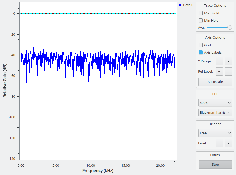 |
That’s not what you want to see when trying to make accurate measurements.
Noise is well behaved over time, though. The trick is to give it time by averaging a lot of measurements.
GNU Radio has averaging functions built in. They can reduce that wild mess to this much cleaner plot:
| Not as noisy noise |
|---|
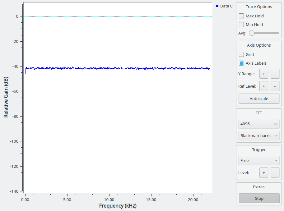 |
That’s still not as clean as I want it, and its not as clean as I got it. I have a few tricks up my sleeve that GNU Radio has heard of, and some that it hasn’t.
One trick that I used is a median filter on the spectrum data before averaging. That greatly smooths the plot for one block of measurements.
The other trick is one that GNU Radio doesn’t have. It is related to a moving average filter, but isn’t (quite) the same. I call it a “walking average filter.” It takes the difference between an existing value and a new value and multiplies the difference by some small value (less than 1.) It then adds that product to the original value. It does much the same job and has much the same effect as a regular moving average, but it has a few advantages over the standard GNU Radio moving average.
Not so important in this day and age, but a large consideration back when I first started doing this kind of thing is the lower memory usage. Rather than keep the last 100 (or whatever number) of spectrum blocks in memory, the walking average never has more than two at a time.
The really nice thing about the walking average, though, is that it produces an output immediately. You see it beginning to move and converge to its average from the very beginning. The standard GNU Radio moving average doesn’t produce any output until it has as many blocks in its memory as you told it to use. If you are using many large blocks of audio, it can take a very long time before you see anything at all.
I tried, but failed to implement the walking average with standard GNU Radio Companion blocks in the GUI. I eventually gave up and implemented it in a Python block. That doesn’t sound like it’d be very fast, but you never use plain Python for this kind of stuff. You use the NumPy library for fast math. Python pretty much just pushes pointers around and asks NumPy to do things.
While I was at it, I put the median filter in the Python block. SciPy has one that suits me better than the standard one in GNU Radio.
That’s pretty much it. Generate white noise, capture two audio channels, do two spectrum analysis, do a bit of math, do some averaging, repeat.
You might notice that nowhere in all of that do I try to calibrate anything. Despite that, the results are within 0.1 ohms when testing a resistor with the impedance tester and comparing to the measured value with an ohmmeter.
There are two tricks that go into that.
One trick is that it doesn’t matter what units the measurements are made in. Look at the math. You have a voltage divided by a voltage. The units cancel, so it is just a ratio. The nameless units of the sound card samples work just as well as volts, so I don’t have to figure out volts from samples.
The other is that I am counting on the analog to digital converters on the line-in of the soundcard to be identical as far as amplification and frequency response go. They generally are, at least to the point that the differences between the two channels are smaller than all the other sources of error. I mean, I can only measure the series resistor to 0.1 ohms. That’s 0.5 %. The sound card channels will be far more identical than that.
Given all of the above, I wouldn’t call the simple impedance tester a precision test tool.
Still, it works and is precise enough to detect tiny variations in impedance - though you can’t really say it is accurate in an absolute sense.
As an example of how well the filtering tames the noise, here’s the impedance of an eight ohm speaker. This is a little 2 inch, low power speaker I had kicking around in the junk drawer.
| 8 ohm speaker impedance plot |
|---|
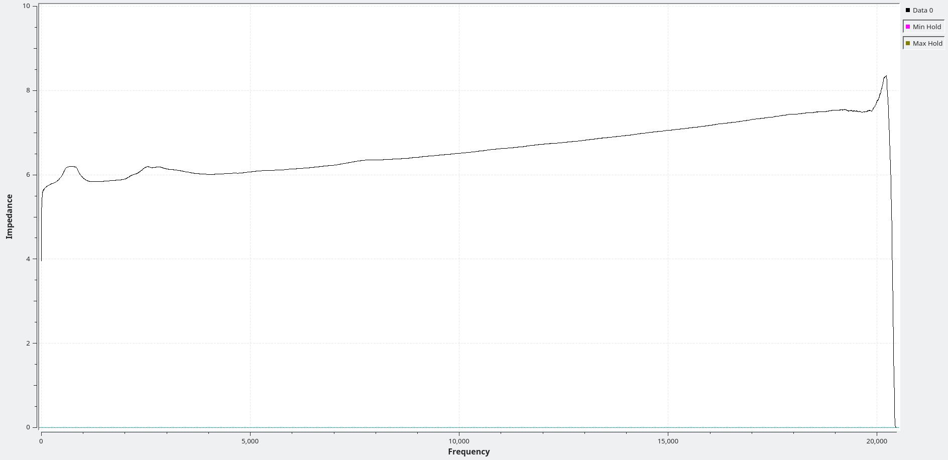 |
Nice and smooth, and clear enough to see a couple of little resonance bumps at around 800 Hz and 2.5kHz.
At any rate, that’s the math and the software behind the simple impedance tester.
The hardware is easier to explain, but I’ll do that another time.